Visualising Black Box Optimisation Problems in Machine Learning

Black box optimisation in Machine Learning is a pretty common scenario. More often than not, the process or model we are trying to optimise does not have an algebraic model that can be solved analytically.

Moreover, in certain use cases where the objective function is expensive to evaluate, a general approach consists of creating a simpler surrogate model of the objective function ,which is cheaper to evaluate and will be used instead to solve the optimisation problem.

This Python tutorial shows how you can evaluate and visualise your Gaussian Process surrogates with Mind Foundry Optimise, an API for Bayesian Optimisation.

In this tutorial, we're going to use Mind Foundry Optimise to find the global minimum of the Beale function defined by the following formula: 

Installation

Mind Foundry Optimise is on PyPi and can be pip installed directly:

!pip install mindfoundry-optaas-client

%matplotlib inline
from matplotlib import pyplot as plt
import numpy as np

from mindfoundry.optaas.client.client import OPTaaSClient, Goal
from mindfoundry.optaas.client.parameter import FloatParameter

Connect to Mind Foundry

In order to connect to Mind Foundry you will need an API key which is available with a license to the Mind Foundry Platform.

client = OPTaaSClient(OPTaaS_URL, OPTaaS_API_key)

Create a task

To start the optimization procedure we need to define the parameters and create a task.

parameters = [
    FloatParameter(name='x', minimum=-4.5, maximum=4.5),
    FloatParameter(name='y', minimum=-4.5, maximum=4.5),
]

initial_configurations = 5

task = client.create_task(
    title='Beale Optimization', 
    parameters=parameters, 
    goal=Goal.min,
    initial_configurations=initial_configurations,
    
    
)

configurations = task.generate_configurations(initial_configurations)

We then need to generate some initial uniformly sampled configurations (5) to weight the Gaussian Process surrogate model.

For the purpose of the tutorial, we are going to break the black box optimisation process down into steps. In a typical scenario, we would simply run the task for a total number of iterations.

Run the task for five iterations

number_of_iterations = 5

for i in range(number_of_iterations): 
    configuration = configurations[i]
    x = configuration.values['x']
    y = configuration.values['y']
    score = beale_function(x, y) 
    next_configuration = task.record_result(configuration=configuration, score=score)
    configurations.append(next_configuration)

Now that we have weighted the surrogate model with the initial configurations, we are going to retrieve its values to visualise it.

Retrieving the surrogate

We are going to request predictions from the surrogate model generated by Mind Foundry. The predictions of the Gaussian Process surrogate model are characterised by their mean and variance.

random_configs_values = [{'x': np.random.uniform(-4.5, 4.5), 
                          'y': np.random.uniform(-4.5, 4.5)
                          } for _ in range(1000)]

predictions = task.get_surrogate_predictions(random_configs_values)

mean = [p.mean for p in predictions]
var = [p.variance for p in predictions]

We are now going to retrieve the evaluations of the Beale function for the initial 5 configurations:

predictions = task.get_surrogate_predictions(random_configs_values)

surrogate_X = [[c['x'], c['y']] for c in random_configs_values]
surrogate_X=np.array(surrogate_X)

results = task.get_results(include_configurations=True)

evaluations_config_values = [r.configuration.values for r in results]
evaluations_score = [r.score for r in results]

Plotting the surrogate

We are now going to reformat the values to plot them:

xs = [results[i].configuration.values['x'] for i in range(len(results)) ]
ys = [results[i].configuration.values['y'] for i in range(len(results)) ]
zs=evaluations_score

beale=np.zeros(len(surrogate_X[:,1]))

for i in range(len(surrogate_X[:,1])):
    beale[i]=beale_function(surrogate_X[i,0], surrogate_X[i,1])

And finally we are going to plot the surrogate vs the real function and superpose the plots with the function evaluations made by Mind Foundry.

plt.clf()
fig = plt.figure(figsize=(20, 10))
ax3d = fig.add_subplot(1, 2, 1, projection='3d')
ax3d.view_init(15, 45)

surface_plot = ax3d.plot_trisurf(surrogate_X[:,0], surrogate_X[:,1], np.array(mean), cmap=plt.get_cmap('coolwarm'), zorder=2, label='Surrogate')
surface_plot.set_alpha(0.28)

plt.title('Surrogate after 5 iterations')
ax3d.plot(xs, ys,zs, 'x', label='evaluations')

plt.xlabel('x')
plt.ylabel('y')

ax3d = fig.add_subplot(1, 2, 2, projection='3d')
ax3d.view_init(15, 45)

surface_plot_real = ax3d.plot_trisurf(surrogate_X[:,0], surrogate_X[:,1], true, cmap=plt.get_cmap('coolwarm'), zorder=2, label='real')
surface_plot_real.set_alpha(0.28)

plt.title('Real')
ax3d.plot(xs, ys,zs, 'x', label='evaluations')

display(plt.gcf())

plt.close('all')

Which outputs:

 

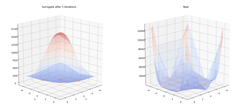
As we can see, the surrogate doesn’t look much like the real function after five iterations, but we expect this to change as it improves its knowledge of the underlying function and the number of evaluations increases.

Evolution of the surrogate

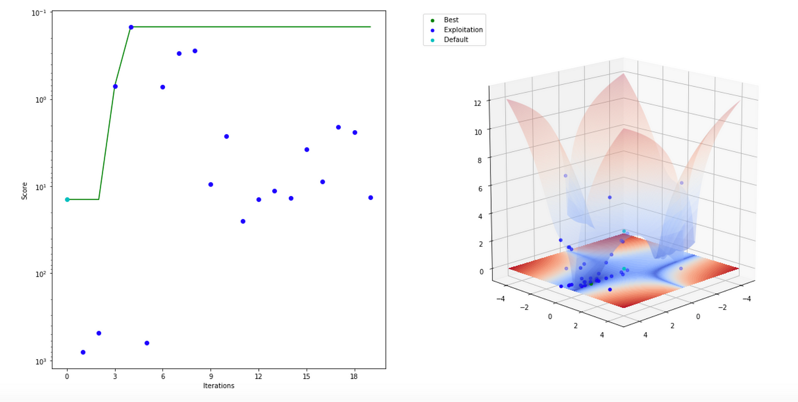
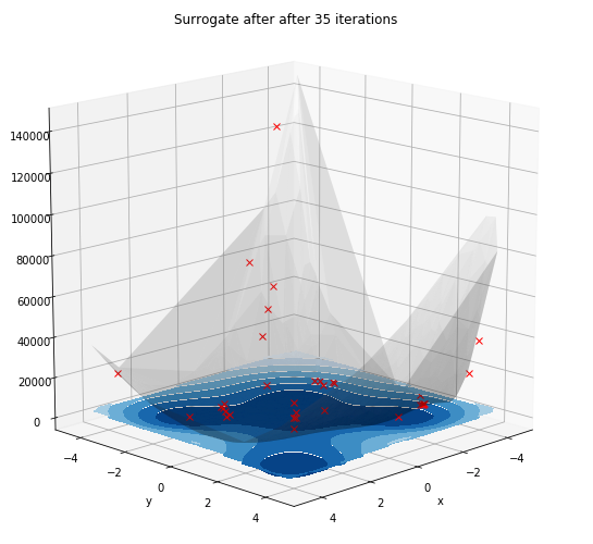
As we increase the number of iterations, the Surrogate quickly adapts to a more realistic representation of the Beale function. These plots were generated with the same code as above.

 

 

 

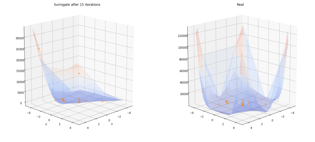
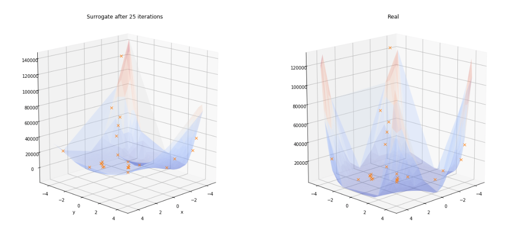
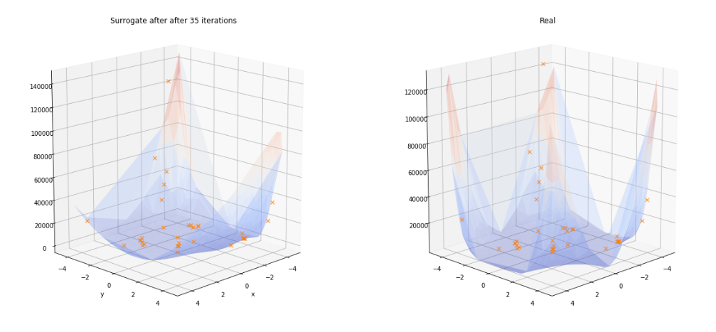
The same procedure from a different angle shows the evolution of the performance of Mind Foundry Optimise and highlights the concentration of recommendations near the optima:

We can also attempt to visualise the variance of the surrogate with a contour plot. The darker shades of blue indicate a low uncertainty of the associated predictions.